Gharsa is a smart AI assistant designed for beginners and plant lovers who want to grow healthy plants but lack expert guidance.

Gharsa’s Eye focuses on detecting and classifying plant leaf diseases using just an image, making plant care more accessible.

In this notebook, I’ll walk you through inventive techniques that tackle two major challenges in the field: the scarcity of labeled data, and the obscurity of small details in zoomed-out images. We’ll use a blend of classic and modern computer vision methods to build a reliable disease detection pipeline from scratch.

This work builds on a CLIP model I finetuned with a classification accuracy of >90%.

We start with installing all required libraries

# First is the SAM library and all of its dependencies
!pip install -q 'git+https://github.com/facebookresearch/segment-anything.git'

# To view SAM masks
!pip install opencv-python matplotlib

# Get a checkpoint of SAM
!wget https://dl.fbaipublicfiles.com/segment_anything/sam_vit_h_4b8939.pth

Set-up

import torch
import torchvision
import sys
import numpy as np
import torch
import matplotlib.pyplot as plt
import cv2

print("PyTorch version:", torch.__version__)
print("Torchvision version:", torchvision.__version__)
print("CUDA is available:", torch.cuda.is_available())
DEVICE = torch.device('cuda:0' if torch.cuda.is_available() else 'cpu')

PyTorch version: 2.6.0+cu124
Torchvision version: 0.21.0+cu124
CUDA is available: True

Helper functions

##1. Disply Annotations show_anns’ credits

def show_anns(anns):
    if len(anns) == 0:
        return
    sorted_anns = sorted(anns, key=(lambda x: x['area']), reverse=True)
    ax = plt.gca()
    ax.set_autoscale_on(False)

    img = np.ones((sorted_anns[0]['segmentation'].shape[0], sorted_anns[0]['segmentation'].shape[1], 4))
    img[:,:,3] = 0
    for ann in sorted_anns:
        m = ann['segmentation']
        color_mask = np.concatenate([np.random.random(3), [0.5]])
        img[m] = color_mask
    ax.imshow(img)

2. Color Masking

Here is a pipeline I created to highlight the possibly diseased areas in the leaf. You can learn how to make one from my blog section found on my medium article.

def color_mask(img_path):
    img = cv2.imread(img_path) # Read the image

    # Convert the color standard to HSV
    hsv = cv2.cvtColor(img, cv2.COLOR_BGR2HSV)

    # Find the leaf
    leaf_mask = cv2.inRange(hsv, (25, 100, 70), (65, 255, 255))

    # Create a black 1-channel image to draw on the leaf mask
    leaf = np.zeros(leaf_mask.shape, dtype=np.uint8)

    # Get the outermost contour
    contours, _ = cv2.findContours(leaf_mask, cv2.RETR_EXTERNAL, cv2.CHAIN_APPROX_SIMPLE)

    # Draw contours on the black image
    cv2.drawContours(leaf, contours, -1, 255, cv2.FILLED)

    # Construct the powdery mildew mask
    mildew_mask = cv2.inRange(hsv, (0, 0, 180), (180,  60, 255))

    # Construct the spots mask
    spot_mask = cv2.inRange(hsv, (10,100,10), (20, 255, 200))

    # Construct the rot mask
    rot_mask1 = cv2.inRange(hsv, (5,10,20), (60,120,100))
    rot_mask2 = cv2.inRange(hsv, (10,100,10), (20, 255, 200))
    rot_mask = cv2.bitwise_or(rot_mask1, rot_mask2)

    # Combine the mildew, spot and rot masks then confine within the leaf - others can appear on edges
    temp_mask = cv2.bitwise_or(mildew_mask, spot_mask)
    temp_mask = cv2.bitwise_or(temp_mask, rot_mask)
    temp_mask = cv2.bitwise_and(leaf, leaf, mask=temp_mask)

    # Construct the burn mask
    burn_mask = cv2.inRange(hsv, (10,100,10), (20, 255, 200))

    # Construct the chlorosis mask
    chlorosis_mask = cv2.inRange(hsv, (20, 150, 150), (37, 255, 255))

    # Combine disease masks
    disease_mask = cv2.bitwise_or(temp_mask, burn_mask)
    disease_mask = cv2.bitwise_or(disease_mask, chlorosis_mask)

    # Smooth out edges and close gaps in mask
    kh, kw = [max(9, int(round(min(img.shape[:2]) * 0.01))) | 1]*2
    kernel = cv2.getStructuringElement(cv2.MORPH_ELLIPSE, (kh, kw))
    disease_mask = cv2.morphologyEx(disease_mask, cv2.MORPH_CLOSE, kernel)
    disease_mask = cv2.morphologyEx(disease_mask, cv2.MORPH_OPEN,  kernel)


    return disease_mask

3. Crop Segments Made by SAM

Function responsible for cropping segments with a minimum size and retaining information.

MIN_SIZE = 256          # smallest crop side you allow

def _cluster_bboxes(bboxes, min_size):
    """
    Greedy one-pass clustering:
        – Start a new cluster for each bbox that cannot fit into an existing one.
        – A bbox fits an existing cluster if the *union* of the two
          is ≤ min_size in both width and height.
    Returns: list of dicts  { "bounds": (x1,y1,x2,y2), "indices": [i,…] }
    """
    clusters = []
    for i, (x1,y1,x2,y2) in enumerate(bboxes):
        placed = False
        for cl in clusters:
            cx1,cy1,cx2,cy2 = cl["bounds"]
            ux1, uy1 = min(cx1,x1), min(cy1,y1)
            ux2, uy2 = max(cx2,x2), max(cy2,y2)
            if (ux2-ux1) <= min_size and (uy2-uy1) <= min_size:
                cl["bounds"]   = (ux1, uy1, ux2, uy2)
                cl["indices"].append(i)
                placed = True
                break
        if not placed:
            clusters.append({"bounds": (x1,y1,x2,y2), "indices":[i]})
    return clusters


def _pad_bounds(bounds, img_w, img_h, min_size):
    """Expand bounds to ≥ min_size each side, clamp to image edges."""
    x1,y1,x2,y2 = bounds
    w, h = x2-x1, y2-y1

    # symmetric padding
    if w < min_size:
        pad = (min_size - w) // 2
        x1 -= pad;  x2 = x1 + min_size
    if h < min_size:
        pad = (min_size - h) // 2
        y1 -= pad;  y2 = y1 + min_size

    # clip to valid coordinates
    x1, y1 = max(0, x1), max(0, y1)
    x2, y2 = min(img_w, x2), min(img_h, y2)

    # if clipping shrank the box below min_size, shift it back
    if x2 - x1 < min_size:
        if x1 == 0:     x2 = min(img_w, min_size)
        else:           x1 = max(0, x2 - min_size)
    if y2 - y1 < min_size:
        if y1 == 0:     y2 = min(img_h, min_size)
        else:           y1 = max(0, y2 - min_size)

    return (x1, y1, x2, y2)


def crop_segments(image: np.ndarray, filtered_masks: list, min_size: int = MIN_SIZE):
    """
    image           : H×W[×C] NumPy array
    filtered_masks  : list of SAM annotations, each containing 'bbox' = [x, y, w, h]
    Returns         : list of dicts: { "crop": np.ndarray, "anns": [ann, …], "bounds": (x1,y1,x2,y2) }
    """
    H, W = image.shape[:2]

    # collect (x1,y1,x2,y2) for every ann
    bboxes = [
        (int(bx), int(by), int(bx+bw), int(by+bh))
        for ann in filtered_masks
        for bx,by,bw,bh in [ann["bbox"]]
    ]

    # greedy clustering so that each cluster fits inside a min_size square
    clusters = _cluster_bboxes(bboxes, min_size)

    # pad each cluster to at least min_size and extract the crop
    crops = []
    for cl in clusters:
        x1,y1,x2,y2 = _pad_bounds(cl["bounds"], W, H, min_size)
        crop_img    = image[y1:y2, x1:x2]
        crop_anns   = [filtered_masks[i] for i in cl["indices"]]

        crops.append({
            "crop"   : crop_img,
            "anns"   : crop_anns,
            "bounds" : (x1,y1,x2,y2),
        })

    return crops

Automatic Mask Generation

Instantiate SAM

We’ll instantiate the mask generator in accordance with our needs. First, we’ll enable it look at more fine grained details in the images (crops) as diseases could sometimes be small (i.e. spots).

from segment_anything import sam_model_registry, SamAutomaticMaskGenerator, SamPredictor

# We'll load the model using the checkpoint we got
sam_checkpoint = "sam_vit_h_4b8939.pth"
model_type = "vit_h"

sam = sam_model_registry[model_type](checkpoint=sam_checkpoint)
sam.to(device=DEVICE)

mask_generator = SamAutomaticMaskGenerator(
    sam,
)

Prepare test images

!mkdir images
!wget -P images https://raw.githubusercontent.com/abodeza/plant_disease_detection/main/test_imgs/Aziz_crop.jpg
!wget -P images https://raw.githubusercontent.com/abodeza/plant_disease_detection/main/test_imgs/mildew.jpg

# We can use the mask generator as such
image_name = "images/mildew.jpg"
image = cv2.imread(image_name)
image_rgb = cv2.cvtColor(image, cv2.COLOR_BGR2RGB)

Mask generation returns a list over masks, where each mask is a dictionary containing various data about the mask. These keys are:

segmentation : the mask
area : the area of the mask in pixels
bbox : the boundary box of the mask in XYWH format
predicted_iou : the model’s own prediction for the quality of the mask
point_coords : the sampled input point that generated this mask
stability_score : an additional measure of mask quality
crop_box : the crop of the image used to generate this mask in XYWH format

more details on their repo

Generate masks

masks = mask_generator.generate(image)

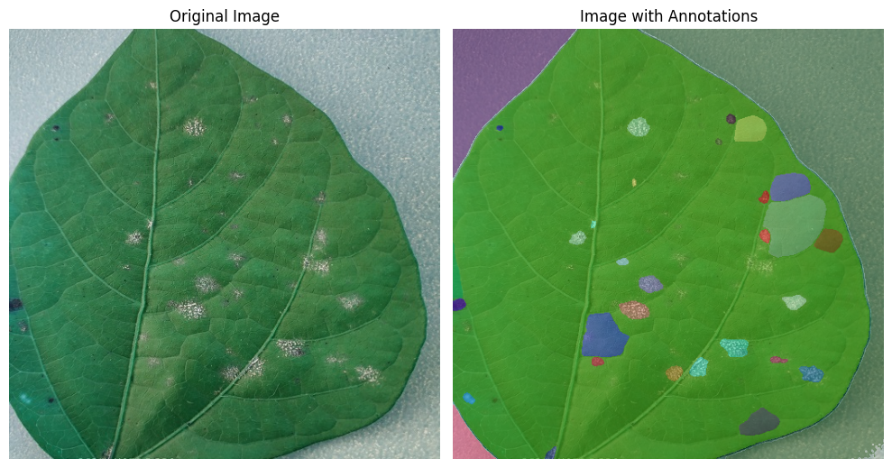
Let’s visualize the automatically generated masks

fig, axes = plt.subplots(1, 2, figsize=(10, 10))

# Left: image only
axes[0].imshow(image)
axes[0].axis('off')
axes[0].set_title("Original Image")

# Right: image + annotations
axes[1].imshow(image)
plt.sca(axes[1])  # set current axis
show_anns(masks)
axes[1].axis('off')
axes[1].set_title("Image with Annotations")

plt.tight_layout()
plt.show()

We can do better

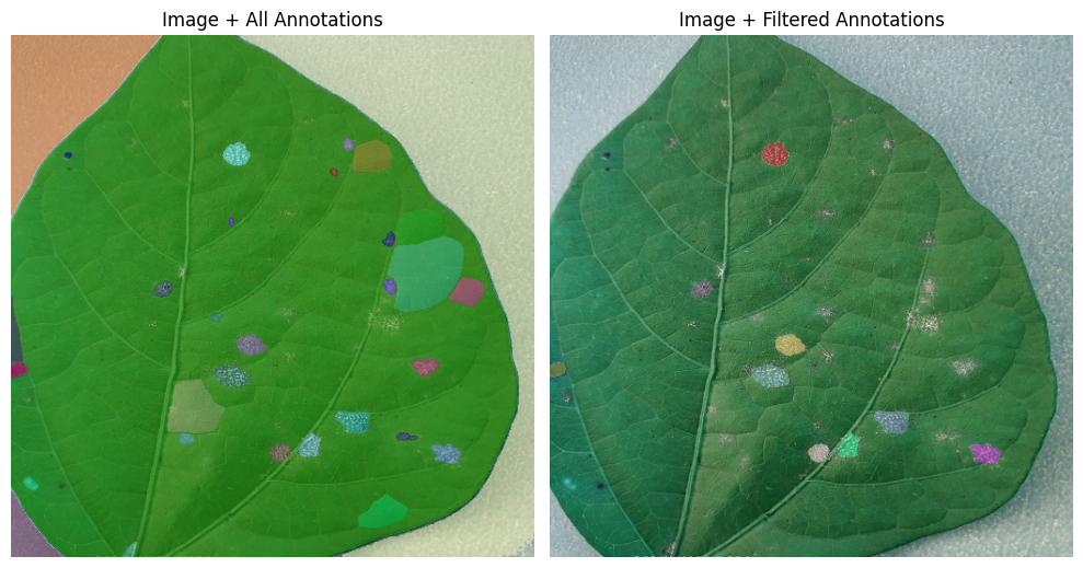
The masks generated by SAM automatically are impressive, but we care mostly about the diseased areas.

We will create a color mask that highlights possibly diseased areas and choose the SAM masks that best align with it.

disease_mask = color_mask(image_name)
filtered_masks = []
for res in masks:
    mask = res["segmentation"].astype("uint8")
    inter = np.count_nonzero(mask & (disease_mask > 0))
    if inter > 0.2 * np.count_nonzero(mask):
        filtered_masks.append(res)               # keep only good masks

fig, axes = plt.subplots(1, 2, figsize=(10, 10))

# Left: image + all annotations
axes[0].imshow(image)
plt.sca(axes[0])  # set current axis
show_anns(masks)
axes[0].axis('off')
axes[0].set_title("Image + All Annotations")

# Right: image + filtered annotations
axes[1].imshow(image)
plt.sca(axes[1])  # set current axis
show_anns(filtered_masks)
axes[1].axis('off')
axes[1].set_title("Image + Filtered Annotations")

plt.tight_layout()
plt.show()

Crop segments for analysis

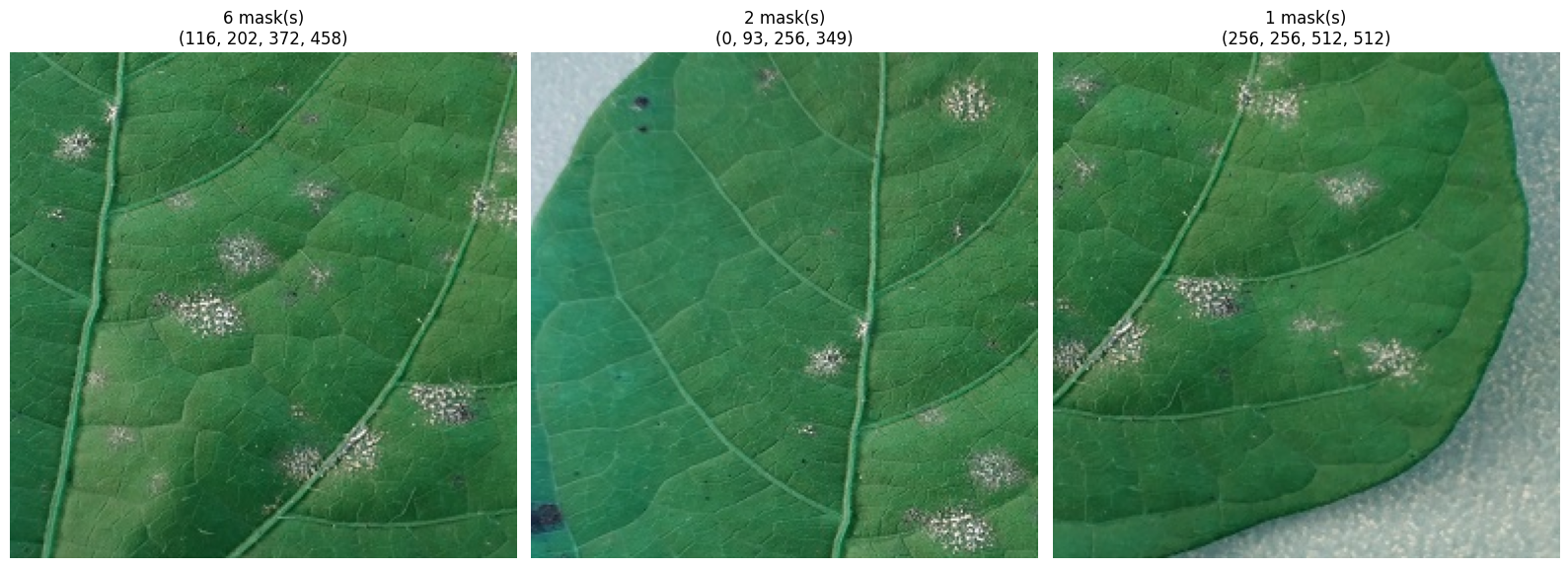
SAM returns the bounding box coordinates for each mask. If we were to crop each segment directly, some might be too small for later analysis. Hence, we’ll ensure the crops are large enough and not overlapping.

crops = crop_segments(image, filtered_masks)

def show_crops(crops, max_cols=4, figsize=(16, 8)):
    """
    crops: output of `crop_segments`, list of dicts with keys 'crop', 'anns', 'bounds'
    max_cols: max number of columns in the plot grid
    """
    num = len(crops)
    cols = min(num, max_cols)
    rows = (num + cols - 1) // cols

    plt.figure(figsize=figsize)
    for i, crop_data in enumerate(crops):
        crop = crop_data['crop']
        anns = crop_data['anns']
        bounds = crop_data['bounds']

        plt.subplot(rows, cols, i+1)
        plt.imshow(crop)
        plt.title(f"{len(anns)} mask(s)\n{bounds}")
        plt.axis('off')

    plt.tight_layout()
    plt.show()
show_crops(crops)

Load and setup CLIP

CLIP is trained on image and textual description pairs. Thus, it’s able to measure the closeness of textual prompts with images.

Furthermore, I have finetuned CLIP on the 5 supported disease classes and ~100 images per class making it better suited for the task.

# 1. PROMPT BANK & LOADING CLIP MODEL
from pathlib import Path
from PIL import Image
import cv2, torch, numpy as np, matplotlib.pyplot as plt
from sentence_transformers import SentenceTransformer

prompt_bank = {
    "Rot":                 ["rot"],
    "Spot":                ["spot"],
    "Burn":                ["burn"],
    "Powdery Mildew":      ["powdery_mildew"],
    "Nutrient Deficiency": ["chlorosis"],
}

flat_prompts  = [p for lst in prompt_bank.values() for p in lst]
prompt_class  = [cls for cls, lst in prompt_bank.items() for _ in lst]

device       = "cuda" if torch.cuda.is_available() else "cpu"
clip_model   = SentenceTransformer("abodeza/clip-ViT-B-32-leaf-disease",
                                   device=device)

with torch.no_grad():
    text_feats = clip_model.encode(flat_prompts,
                                   convert_to_tensor=True,
                                   device=device)
    text_feats = torch.nn.functional.normalize(text_feats, dim=-1)

#  2. CLASSIFY CROPS & SAVE RESULTS
CLIP_THRESH = 0.3          # confidence cut-off
OUT_DIR     = Path("crops_out")
OUT_DIR.mkdir(parents=True, exist_ok=True)

selected = {k: [] for k in prompt_bank}    # store results per class

for j, crop_dict in enumerate(crops):      # ‘crops’ comes from crop_segments
    crop_img  = crop_dict["crop"]          # H×W×C, RGB
    pil_crop  = Image.fromarray(crop_img)

    with torch.no_grad():
        feat   = clip_model.encode([pil_crop], convert_to_tensor=True,
                                   device=device)
        feat   = torch.nn.functional.normalize(feat, dim=-1)
        sims   = (feat @ text_feats.T).squeeze(0)

    best_idx   = int(torch.argmax(sims))
    best_score = float(sims[best_idx])

    if best_score < CLIP_THRESH:
        continue

    cls_name  = prompt_class[best_idx]
    file_name = f"crop_{j:03d}_{cls_name}_{best_score:.2f}.png"
    cv2.imwrite(str(OUT_DIR / file_name),
                cv2.cvtColor(crop_img, cv2.COLOR_RGB2BGR))

    selected[cls_name].append({
        "file":   file_name,
        "score":  best_score,
        "bounds": crop_dict["bounds"],
    })

print(f"{sum(len(v) for v in selected.values())} crops saved at {OUT_DIR.resolve()}")
for cls, lst in selected.items():
    print(f"{cls:20s}: {len(lst)}")

3 crops saved at /content/crops_out
Rot                 : 0
Spot                : 0
Burn                : 0
Powdery Mildew      : 3
Nutrient Deficiency : 0

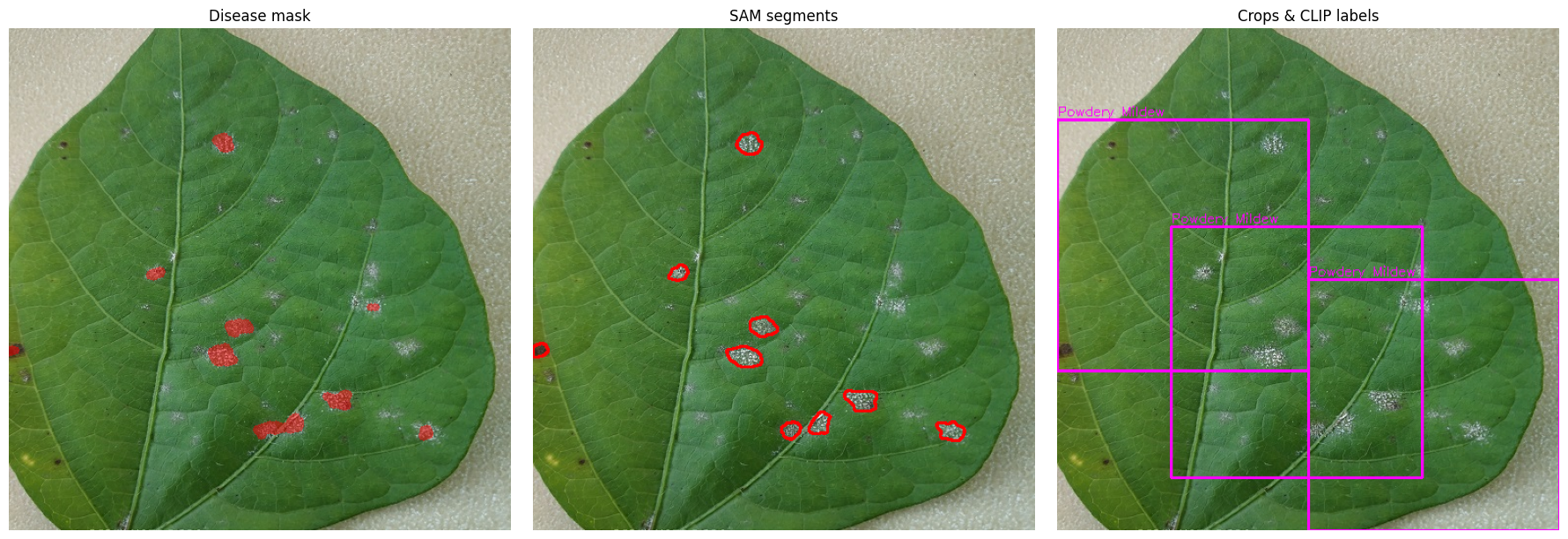
# 3. VISUAL SUMMARY OF THE PIPELINE
fig, axes = plt.subplots(1, 3, figsize=(18, 6))

# (a) Disease-mask overlay
overlay = image_rgb.copy()
overlay[disease_mask > 0] = (
    overlay[disease_mask > 0] * 0.5 + np.array([255, 0, 0]) * 0.5
).astype(np.uint8)
axes[0].imshow(overlay); axes[0].set_title("Disease mask"); axes[0].axis("off")

# (b) SAM segment contours
vis = image_rgb.copy()
for res in filtered_masks:
    cnts, _ = cv2.findContours(res["segmentation"].astype(np.uint8),
                               cv2.RETR_EXTERNAL, cv2.CHAIN_APPROX_SIMPLE)
    cv2.drawContours(vis, cnts, -1, (255, 0, 0), 2)
axes[1].imshow(vis); axes[1].set_title("SAM segments"); axes[1].axis("off")

# (c) Crops + CLIP labels
final_vis = image_rgb.copy()
for cls, lst in selected.items():
    for e in lst:
        x1,y1,x2,y2 = e["bounds"]
        cv2.rectangle(final_vis, (x1, y1), (x2, y2), (255, 0, 255), 2)
        cv2.putText(final_vis, cls, (x1, max(0, y1-4)),
                    cv2.FONT_HERSHEY_SIMPLEX, 0.45, (255, 0, 255), 1)
axes[2].imshow(final_vis); axes[2].set_title("Crops & CLIP labels"); axes[2].axis("off")

plt.tight_layout(); plt.show()

# 4. TOP-SCORING CROPS
TOP_K_VIZ = 5
for cls, lst in selected.items():
    if not lst:
        continue
    lst.sort(key=lambda d: d["score"], reverse=True)
    n = min(len(lst), TOP_K_VIZ)

    plt.figure(figsize=(3*n, 3))
    for i, entry in enumerate(lst[:n]):
        img = cv2.cvtColor(cv2.imread(str(OUT_DIR / entry["file"])),
                           cv2.COLOR_BGR2RGB)
        plt.subplot(1, n, i+1); plt.imshow(img); plt.axis("off")
        plt.title(f"{cls}\n{entry['score']:.2f}", fontsize=8)
    plt.suptitle(f"{cls} – top {n}", fontsize=14)
    plt.tight_layout(); plt.show()

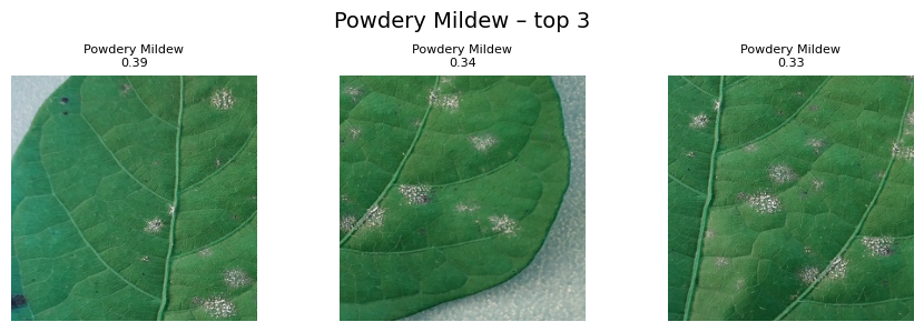
Now we have reached the end of the notebook. We went through color masking, SAM’s automatic mask generation and CLIP’s image-text pairs automating the task of locating, and accurately classifying the diseases on plant leaves.

The next steps are to simplify the pipeline further to fit into one function that can be called once. Additionally, I’m working on producing the same promising results for all the other diseases.

Please don’t hesitate to reach out with any questions!

Gharsa's Eye